RuleFit
目次
RuleFit
Friedman, Jerome H and Bogdan E Popescu. “Predictive learning via rule ensembles.” The Annals of Applied Statistics. JSTOR, 916–54. (2008).(pdf)
実験用のデータを取得する
openmlで公開されている house_sales データセットを使用して回帰モデルを作成します。
※上記openmlページではデータの出典が不明ですが自分が調べた限りではデータの提供元はここのようです。
# Google Colaboratory で実行する場合はインストールする
if str(get_ipython()).startswith("<google.colab."):
    !pip install dtreeviz
    !pip install japanize_matplotlib
import japanize_matplotlib
import matplotlib.pyplot as plt
import pandas as pd
from sklearn.datasets import fetch_openml

dataset = fetch_openml(data_id=42092)
X = pd.DataFrame(dataset.data, columns=dataset.feature_names)
X = X.select_dtypes("number")
y = dataset.target
---------------------------------------------------------------------------
ModuleNotFoundError                       Traceback (most recent call last)
Input In [2], in <cell line: 1>()
----> 1 import japanize_matplotlib
      2 import matplotlib.pyplot as plt
      3 import pandas as pd

ModuleNotFoundError: No module named 'japanize_matplotlib'
# 表示する文字サイズを調整
plt.rc("font", size=20)
plt.rc("legend", fontsize=16)
plt.rc("xtick", labelsize=14)
plt.rc("ytick", labelsize=14)

# 乱数
import numpy as np

np.random.seed(777)
データの中身を確認する
X.head(10)
| bedrooms | bathrooms | sqft_living | sqft_lot | floors | waterfront | view | condition | grade | sqft_above | sqft_basement | yr_built | yr_renovated | lat | long | sqft_living15 | sqft_lot15 | |
|---|---|---|---|---|---|---|---|---|---|---|---|---|---|---|---|---|---|
| 0 | 3.0 | 1.00 | 1180.0 | 5650.0 | 1.0 | 0.0 | 0.0 | 3.0 | 7.0 | 1180.0 | 0.0 | 1955.0 | 0.0 | 47.5112 | -122.257 | 1340.0 | 5650.0 |
| 1 | 3.0 | 2.25 | 2570.0 | 7242.0 | 2.0 | 0.0 | 0.0 | 3.0 | 7.0 | 2170.0 | 400.0 | 1951.0 | 1991.0 | 47.7210 | -122.319 | 1690.0 | 7639.0 |
| 2 | 2.0 | 1.00 | 770.0 | 10000.0 | 1.0 | 0.0 | 0.0 | 3.0 | 6.0 | 770.0 | 0.0 | 1933.0 | 0.0 | 47.7379 | -122.233 | 2720.0 | 8062.0 |
| 3 | 4.0 | 3.00 | 1960.0 | 5000.0 | 1.0 | 0.0 | 0.0 | 5.0 | 7.0 | 1050.0 | 910.0 | 1965.0 | 0.0 | 47.5208 | -122.393 | 1360.0 | 5000.0 |
| 4 | 3.0 | 2.00 | 1680.0 | 8080.0 | 1.0 | 0.0 | 0.0 | 3.0 | 8.0 | 1680.0 | 0.0 | 1987.0 | 0.0 | 47.6168 | -122.045 | 1800.0 | 7503.0 |
| 5 | 4.0 | 4.50 | 5420.0 | 101930.0 | 1.0 | 0.0 | 0.0 | 3.0 | 11.0 | 3890.0 | 1530.0 | 2001.0 | 0.0 | 47.6561 | -122.005 | 4760.0 | 101930.0 |
| 6 | 3.0 | 2.25 | 1715.0 | 6819.0 | 2.0 | 0.0 | 0.0 | 3.0 | 7.0 | 1715.0 | 0.0 | 1995.0 | 0.0 | 47.3097 | -122.327 | 2238.0 | 6819.0 |
| 7 | 3.0 | 1.50 | 1060.0 | 9711.0 | 1.0 | 0.0 | 0.0 | 3.0 | 7.0 | 1060.0 | 0.0 | 1963.0 | 0.0 | 47.4095 | -122.315 | 1650.0 | 9711.0 |
| 8 | 3.0 | 1.00 | 1780.0 | 7470.0 | 1.0 | 0.0 | 0.0 | 3.0 | 7.0 | 1050.0 | 730.0 | 1960.0 | 0.0 | 47.5123 | -122.337 | 1780.0 | 8113.0 |
| 9 | 3.0 | 2.50 | 1890.0 | 6560.0 | 2.0 | 0.0 | 0.0 | 3.0 | 7.0 | 1890.0 | 0.0 | 2003.0 | 0.0 | 47.3684 | -122.031 | 2390.0 | 7570.0 |
RuleFitを実行する
Python implementation of the rulefit algorithm - GitHubの実装を使用してRuleFitを動かしてみます。
※実行する際は import warnings;warnings.simplefilter('ignore') は外してください
from rulefit import RuleFit
import warnings

warnings.simplefilter("ignore")  # ConvergenceWarning

rf = RuleFit(max_rules=100)
rf.fit(X.values, y, feature_names=list(X.columns))
RuleFit(max_rules=100,
        tree_generator=GradientBoostingRegressor(learning_rate=0.01,
                                                 max_depth=100,
                                                 max_leaf_nodes=5,
                                                 n_estimators=28,
                                                 random_state=27,
                                                 subsample=0.04543939429397564))
作成されたルールを確認する
rules = rf.get_rules()
rules = rules[rules.coef != 0].sort_values(by="importance", ascending=False)
rules.head(10)
| rule | type | coef | support | importance | |
|---|---|---|---|---|---|
| 8 | grade | linear | 6.199314e+04 | 1.000000 | 66184.725645 |
| 29 | sqft_living > 9475.0 | rule | 1.927942e+06 | 0.001018 | 61491.753935 |
| 43 | grade > 8.5 & sqft_living > 3405.0 & long <= -... | rule | 3.570118e+05 | 0.024440 | 55126.384264 |
| 2 | sqft_living | linear | 5.532732e+01 | 1.000000 | 46347.924165 |
| 11 | yr_built | linear | -1.522004e+03 | 1.000000 | 44393.726859 |
| 15 | sqft_living15 | linear | 5.344916e+01 | 1.000000 | 34501.058499 |
| 62 | lat <= 47.516000747680664 & sqft_living <= 3920.0 | rule | -6.549757e+04 | 0.361507 | 31467.457947 |
| 103 | sqft_basement <= 3660.0 & grade > 9.5 | rule | 1.240216e+05 | 0.068228 | 31270.434139 |
| 48 | sqft_living <= 9475.0 & grade > 9.5 & long > -... | rule | -1.473030e+05 | 0.040733 | 29117.596559 |
| 67 | sqft_living <= 4695.0 & waterfront > 0.5 & sqf... | rule | 3.936285e+05 | 0.005092 | 28016.079499 |
ルールが正しいか確認してみる
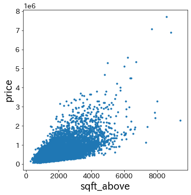
sqft_above linear 8.632149e+01 1.000000 66243.550192 のルールに基づいて、sqft_above が増加すると y(price)が増える傾向にあるかどうか確認します。
plt.figure(figsize=(6, 6))
plt.scatter(X["sqft_above"], y, marker=".")
plt.xlabel("sqft_above")
plt.ylabel("price")
Text(0, 0.5, 'price')
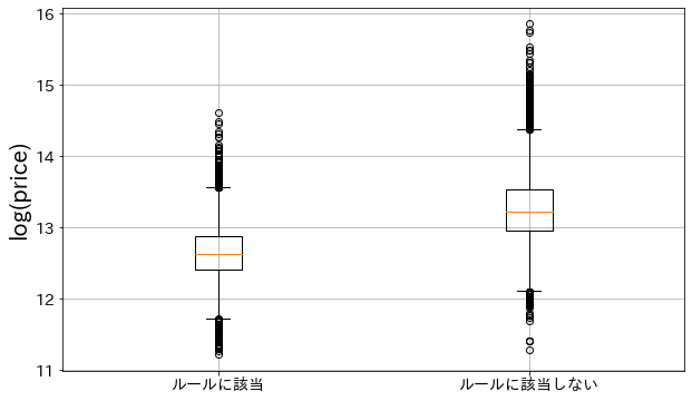
sqft_living <= 3935.0 & lat <= 47.5314998626709 rule -8.271074e+04 0.377800 40101.257833 のルールに該当するデータのみ抽出してみます。
係数がマイナスになっているので、このルールに該当するデータのy(price)は低い傾向にあるはずです。
log(y)を箱髭図で確認すると、確かにルールに該当しているデータのyはルールに該当しないデータのyと比較すると低くなっています。
applicable_data = np.log(
    y[X.query("sqft_living <= 3935.0 & lat <= 47.5314998626709").index]
)
not_applicable_data = np.log(
    y[X.query("not(sqft_living <= 3935.0 & lat <= 47.5314998626709)").index]
)

plt.figure(figsize=(10, 6))
plt.boxplot([applicable_data, not_applicable_data], labels=["ルールに該当", "ルールに該当しない"])
plt.ylabel("log(price)")
plt.grid()
plt.show()