リッジ回帰とラッソ回帰
目次
リッジ回帰とラッソ回帰
# Google Colaboratory で実行する場合はインストールする
if str(get_ipython()).startswith("<google.colab."):
    !pip install japanize_matplotlib
import numpy as np
import matplotlib.pyplot as plt
import japanize_matplotlib
from sklearn.datasets import make_regression
from sklearn.linear_model import LinearRegression, Ridge, Lasso
from sklearn.model_selection import cross_val_score
from sklearn.pipeline import make_pipeline
from sklearn.preprocessing import StandardScaler
---------------------------------------------------------------------------
ModuleNotFoundError                       Traceback (most recent call last)
Input In [2], in <cell line: 2>()
      1 import numpy as np
----> 2 import matplotlib.pyplot as plt
      3 import japanize_matplotlib
      4 from sklearn.datasets import make_regression

ModuleNotFoundError: No module named 'matplotlib'
# 表示する文字サイズを調整
plt.rc("font", size=20)
plt.rc("legend", fontsize=16)
plt.rc("xtick", labelsize=14)
plt.rc("ytick", labelsize=14)

# 乱数
np.random.seed(777)
実験用の回帰データを作成
予測に必要な特徴量 = 2次元(
n_informative= 2)冗長な特徴量あり
n_features = 5
n_informative = 2
X, y = make_regression(
    n_samples=500,
    n_features=n_features,
    n_informative=n_informative,
    noise=0.5,
    random_state=777,
)
X = np.concatenate([X, np.log(X + 100)], 1)  # 冗長な特徴量を追加する
y_mean = y.mean(keepdims=True)
y_std = np.std(y, keepdims=True)
y = (y - y_mean) / y_std
最小二乗法・リッジ回帰・ラッソ回帰モデルを学習
ヒント
それぞれのモデルについて、同じデータをつかって訓練します。
lin_r = make_pipeline(StandardScaler(with_mean=False), LinearRegression()).fit(X, y)
rid_r = make_pipeline(StandardScaler(with_mean=False), Ridge(alpha=2)).fit(X, y)
las_r = make_pipeline(StandardScaler(with_mean=False), Lasso(alpha=0.1)).fit(X, y)
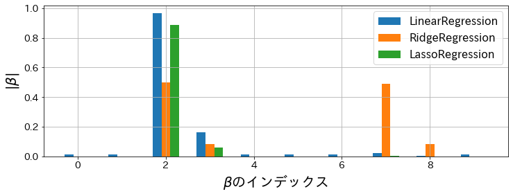
各モデルの係数の値を比較
各係数の絶対値をプロットします。線形回帰は係数がほとんど0にならないことがグラフから見て取れます。 また、Lasso回帰は予測に必要な特徴量以外で係数=0になっていることが確認できます。
feat_index = np.array([i for i in range(X.shape[1])])

plt.figure(figsize=(12, 4))
plt.bar(
    feat_index - 0.2,
    np.abs(lin_r.steps[1][1].coef_),
    width=0.2,
    label="LinearRegression",
)
plt.bar(feat_index, np.abs(rid_r.steps[1][1].coef_), width=0.2, label="RidgeRegression")
plt.bar(
    feat_index + 0.2,
    np.abs(las_r.steps[1][1].coef_),
    width=0.2,
    label="LassoRegression",
)

plt.xlabel(r"$\beta$のインデックス")
plt.ylabel(r"$|\beta|$")
plt.grid()
plt.legend()
<matplotlib.legend.Legend at 0x7fede15ef4c0>